8 Useful Spreadsheet Hacks for Clued Up Project Management

This blog is going to teach you a few spreadsheet hacks, tips, and tricks for managing large projects using Excel. Now, before we get too far into this, let’s address the elephant in the room. It’s 2021, why are we talking about Excel when dedicated project management tools like Trello, Asana, and Monday exist?
Well… sometimes you can’t beat a simple spreadsheet.
Fancy tools like Monday are great for complex projects with lots of moving parts and team members, but if you need to create and manage huge lists of data (photography shot lists, for example), Excel and its copycats are the way to go. It’s worth noting here that all the functionality we’re about to go through works more or less the same way in Google Sheets. Most functions even have the same name, but you might have to do a bit of digging through Google Sheets’ dropdown menus to find them.
So, without further ado, here are a few spreadsheet hacks for managing reams of data. Some of these you’ll probably already know, so here’s a quick list of what’s coming up.
The Spreadsheet Hacks You’ll Learn:
- Sorting Data By Different Columns
- Quickly Sum Long Lists of Figures
- Quick Reference Corner Counters
- Conditional Formatting to Track Project Status
- Creating Dropdown Lists of Project Stages
- Using Concatenate to Automate File Name Creation
- Find & Replace to Save Time
- Freezing Headers and Column Names to Keep Them Onscreen
Sorting Data By Different Columns
You probably already know about sorting in Excel. Head up to the top right corner of the HOME tab and you’ll see the usual Sort & Filter buttons. Using these you can sort by number or arrange by alphabetical. But did you know you can use this on specific data selections?
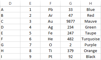
If you highlight only the data you want to sort, then use these buttons, it’ll sort only the highlighted data, leaving cells around it untouched.
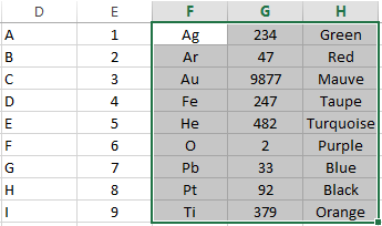
By default, Excel will sort by the first highlighted column, but if you hit TAB on your keyboard you’ll be able to sort using the second column. Keep hitting TAB until you’ve got the column you want to sort by.
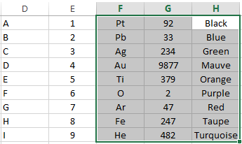
This way you can rearrange data in seconds, without having to copy and paste to ensure the data you want to use to sort is in the first highlighted column.
Quickly Sum Long Lists of Figures
Here’s a quick one. You’ll already know, I’m sure, that you can use a formula to SUM data. Let’s imagine you have ten numbers you want to add together in cells A1 to A10. Normally, you’d go to another cell and type =SUM(A1:A10) to add them together. But there’s an even faster way.
Go to cell A11. Hold ALT and press =
Voila. Excel has automatically summed every cell above A11.
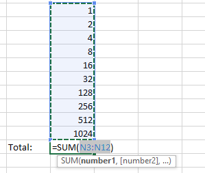
Note though, that it’ll only sum an unbroken chain of cells. If A5 was blank, this shortcut would only add cells A6 to A10 automatically. Try it out.
Quick Reference Corner Counters
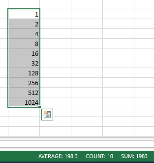
Excel comes with a few built-in features designed to save you time if you just want to quickly SUM, COUNT, or AVERAGE data. Simply highlight the data you want to know more about, then look in the bottom right of the window.
Sum = The highlighted data added together (only works with numbers)
Count = The number of highlighted cells that aren’t blank
Average = The average value for the highlighted cells (only works with numbers)
Personally, I find the quick count feature particularly useful for finding out the number of shots in a shot list. Say I had a mixed shot list of jewellery, apparel, and accessories products, and I want to know how many jewellery shots need to be done. I could selective sort to put all the jewellery shots together, then highlight the names of the jewellery shots. Excel tells me how many there are in the bottom right.
Conditional Formatting to Track Shot Status
Now we’re getting to the good stuff. There’s a lot you can do with conditional formatting, too much to talk about here, but today I’m going to show you a really simple use case.
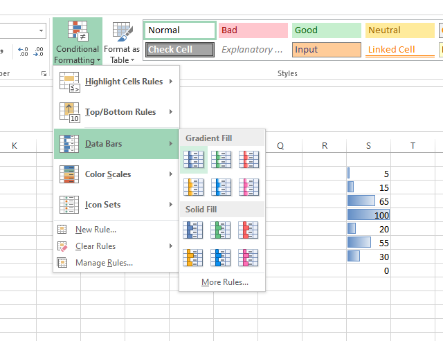
Say you want to colour code cells according to what’s in them. There are a few simple ways to do that, instantly adding a visual element to your data. Simply highlight the cells, click Conditional Formatting on the HOME tab, then click either Data Bars or Colour Scales.
If you want to get more complex than that, here’s a way you can link certain colours to certain values. Let’s say you have a column on a shot list that says YES or NO depending on whether the shot has been edited. Imagine you want the cell to go green if YES, and red if NO. Here’s what you do:
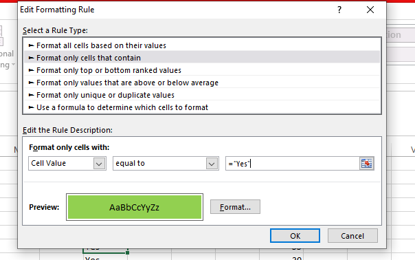
Highlight the top cell in the row, then click Conditional Formatting, then New Rule. A new window will open. Choose “Format Only Cells That Contain”, change the dropdown so that it reads “equal to”, and then type YES in the box to the right of that. At the bottom of the conditional formatting window, click the “Format…” button, and choose a green fill colour.
Hit okay, and that’s that. Copy the cell you’ve just edited, highlight the entire column, then right click and choose to Paste Formatting.
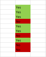
Voila. Done. Then repeat the process with NO, giving it a red colour.
Creating Dropdown Lists of Project Stages
One of the headaches with using Conditional Formatting as outlined above is that it relies on exact data being input. If people don’t use the spreadsheet properly, it all falls apart. Using the Conditional Formatting tip as an example, if someone typed Y rather than YES, the cell wouldn’t go green. This is where dropdown lists are useful.
Dropdown lists are a form of data validation, and you can set it up so that people can only fill in a cell from a pre-set list of options. A dropdown list.
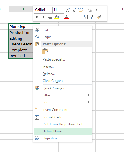
We recommend creating your list on a separate sheet. Add a new sheet in the bottom left, then type each item for your dropdown list into a new cell, keeping it all in one column. Highlight your list, right click, and choose “Define name”. Input a sensible name (in this case, I’m calling it “Status”), then click OK.
Now go back to your main spreadsheet. Highlight the cell (or cells) that you want to use your dropdown list, then go to the Data tab, and click Data Validation, followed by Data Validation…
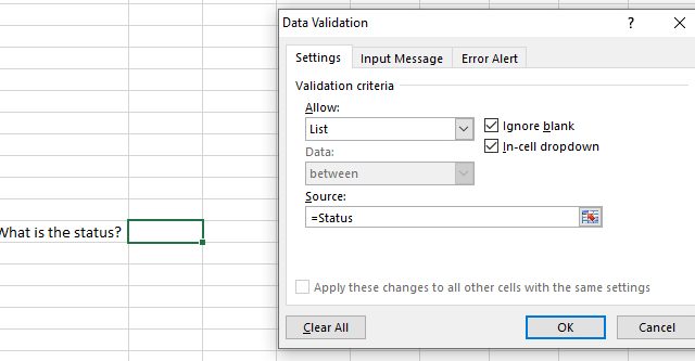
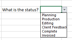
Under the “Allow” heading, select “List”. Then type the name of your list in the bottom box, and hit OK. And there you go. All the cells you highlighted should now only allow information from the dropdown list.
Using Concatenate to Automate File Name Creation
This is my favourite tip, and is particularly useful for creating loads of file names in a ridiculously short amount of time.
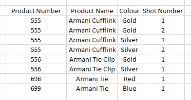
Let’s say you’ve got a shot list with 200 shots on it. Data for each shot is split across four columns:
Product number
Product name
Colour
Shot number (some products have multiple shots)
Now, you could go through and write out the desired file name for each shot, but it would take hours and your fingers might fall off out of boredom. Instead, use Concatenate, and it’ll take you seconds. Here’s an example of how it works:
Imagine we have this data in cells A2, B2, C2, and D2.
555 (this is the product number)
Armani Cufflink (this is the product name)
Gold (this is the product colour)
1 (this is the shot number)
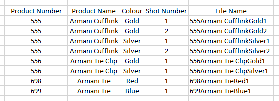
Now, in E5, we type this:
=CONCATENATE(A2,B2,C2,D2)
And get: 555Armani CufflinkGold1
Click and drag this formula down and it’ll automatically create file names for every shot below.
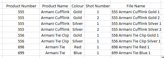
But it doesn’t look very neat, does it? We need to add some spaces between each bit of data to keep it distinct and easy to read. Modify the formula like this:
=CONCATENATE(A2,” “,B2,” “,C2,” “,D2)
This gives: 555 Armani Cufflink Gold 1
Drag it down again, and it’ll give every shot the same treatment. The “ “ simply tells the formula to add a space between each cell’s data. You could write anything between the speech marks and it would add it as plain text between the concatenated cell data.
Find And Replace to Save Time
This one’s dead simple. Imagine someone’s sent you a list of data filled with incorrect terminology, or double spaces between words (grrrr, please don’t do this!)
Highlight the data with the problem, then go to the top right of the HOME tab. Click Find & Select, then Replace. Input the data that needs replacing in the top box, and the data to place it with in the bottom box. Hit “replace all”, and it’ll replace those terms across your whole sheet.
It’s useful for correcting terminology (e.g. replacing photograph with shot) or for tweaking formatting. For example, if you were creating a load of filenames but wanted to replace all of the spaces with dashes, you could use this tool.

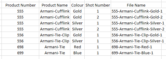
Think carefully before you use this, as there could be unintended consequences. If you wanted to do things the other way around and replace all dashes with spaces, you’d find that the dashes in any hyphenated words are replaced too.
Freezing Headers and Column Names to Keep Them Onscreen
And finally, you can freeze panes to keep information along the top and/or left of your screen constant. If you have a long list of product names, numbers, colours, and references, you’ll find that the column headings disappear as you scroll down. This could lead to confusion.
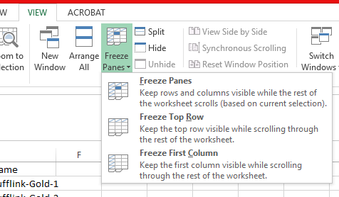
To fix the column names at the top of the screen, go to the View tab and click Freeze Panes. Choose to freeze the top row. Done. Nice and easy.
You can also freeze the left-most column, or use the Freeze Panes option to freeze anything above and to the left of the currently selected cell.
Any Spreadsheet Hacks We’ve Missed
Are there any spreadsheet hacks we’ve missed? Anything you find particularly useful? We’d love to hear from you. And if you’d like to work with an agency that uses every tool at its disposal to keep your projects on track and on budget, please get in touch or head to our LinkedIn page.
Related Posts
-

Making A Difference: Creating Content to Drive Action for Good
April 27, 2023 -

Tom’s Marketing Tales: Client product photography dissected and explained
June 24, 2022 -

Play as Part of the Creative Process
May 17, 2022